The End-to-End Deep Learning: A Beginner's Guide

Deep learning is a subset of machine learning that uses multilayered artificial neural networks to enable computers to learn from massive amounts of data and perform complex tasks that typically require human intelligence, such as image and speech recognition.

How Deep Learning Works
Deep learning models are built on neural networks, which are inspired by the structure and function of the human brain's interconnected neurons. These networks consist of multiple layers of nodes (neurons):
Input Layer: Receives the initial raw data, such as pixel values of an image or words in a sentence.
Hidden Layers: These intermediate layers perform complex mathematical operations (using activation functions) to transform the input data into progressively more abstract and composite representations. The term "deep" refers to the presence of multiple (often numerous) hidden layers.
Output Layer: The final layer produces the model's ultimate prediction or classification.
During training, which requires large amounts of data and high-performance computing power (often GPUs), the network adjusts the "weights" (strength of connections between neurons) and "biases" to minimize the difference between its predictions and the actual desired outputs. This optimization is typically done using algorithms like backpropagation and gradient descent.
Key Neural Network Architectures
CNN
LSTM
RNN
ANN
Transformer Model
GAN (Generative Adversarial Network)
Key Frameworks
Pytorch
Tensorflow
Keras
OpenCV
Convolutional Neural Network (CNN)
A Convolutional Neural Network (CNN or ConvNet) is a specialized deep learning architecture designed to process and analyze visual data like images and video. CNNs excel at automatically extracting hierarchical features (e.g., edges, shapes, and textures) from raw pixel data without manual intervention, making them the de-facto standard for computer vision tasks.
How CNNs Work
The architecture of a CNN is inspired by the human visual cortex and is composed of a series of layers that transform the input data into a final output (e.g., a classification label). The primary layers are:
Convolutional Layer: This core layer applies learnable filters (or kernels) across the input image. Each filter performs a mathematical operation (convolution) to produce a feature map that highlights the presence of specific patterns, such as edges or corners, in different regions of the image. The same weights are shared across the entire image, which dramatically reduces the number of parameters needed.
Activation Function (ReLU): After a convolution operation, a non-linear activation function, typically the Rectified Linear Unit (ReLU), is applied to the feature map. This introduces non-linearity into the model, allowing it to learn more complex patterns.
Pooling Layer: This layer reduces the spatial dimensions (width and height) of the feature maps through a process called down-sampling, most commonly using max pooling. This makes the network more computationally efficient, less prone to overfitting, and helps the model become more robust to the exact position of objects in the image (translational invariance).
Fully Connected Layer: After several rounds of convolution and pooling, the data is flattened into a single one-dimensional vector and passed to a traditional fully connected neural network. This layer uses the high-level features extracted by the previous layers to perform the final classification or prediction task.
What exactly happens in a convolutional layer?
In a convolutional layer, a learnable filter (or kernel) slides over the input data, performing an element-wise multiplication and summation operation at each location to extract specific features such as edges, textures, or shapes. The result of this process is a feature map (or activation map) that indicates where and how strongly the detected feature is present in the input.
Step-by-Step Breakdown
Input Data: The layer receives input, such as an image represented as a matrix of pixel values (e.g., width x height x 3 channels for an RGB image).
Filter Application: A small, pre-defined or randomly initialized filter (e.g., a 3x3 matrix of weights) is placed over a small, local section of the input data, known as the receptive field.
Element-wise Multiplication and Summation: The values in the filter are multiplied by the corresponding pixel values in the receptive field of the input. All these products are then summed together into a single number. This number becomes a single pixel value in the output feature map.
Sliding (Stride): The filter then slides across the input data, typically one pixel at a time (stride of 1), and repeats the multiplication and summation process. The stride determines the step size the filter takes; a larger stride reduces the size of the output feature map.
Creating the Feature Map: This process continues until the filter has covered the entire input's width and height. The collected sum values form the 2D feature map. A CNN typically uses multiple different filters in a single layer, each designed to detect a different pattern, resulting in multiple feature maps stacked together to form an output volume.
Activation Function: After the convolution operation, a non-linear activation function, usually the Rectified Linear Unit (ReLU), is applied to every value in the feature map. This introduces non-linearity, allowing the network to learn more complex relationships.

Key Concepts
Weight Sharing: The same filter (set of weights) is used for all locations in the input image. This dramatically reduces the number of parameters needed compared to a fully connected network and makes the model robust to where features appear in the image (translation invariance).
Local Connectivity: Each neuron in the convolutional layer is only connected to a small, local area of the previous layer, mimicking the structure of the human visual cortex.
Padding: To prevent the feature maps from shrinking with each layer and to ensure that information at the borders of the image is not lost, extra pixels (usually zeros) can be added around the input image boundary before convolution (known as "same" padding).
Learning: The values within the filters are not fixed manually (except in basic image processing examples) but are learned automatically during the network's training process through backpropagation and gradient descent to best extract features relevant to the specific task (e.g., identifying a "dog" vs. a "cat").
LSTM (Long Short-Term Memory)
A Long Short-Term Memory (LSTM) network is an advanced type of recurrent neural network (RNN) specifically designed to effectively learn and remember long-term dependencies in sequential data, such as text, speech, or time series.
Traditional RNNs often suffer from the "vanishing gradient problem," where information from distant past steps is effectively forgotten over time, making it difficult to learn long-range patterns. LSTMs solve this by incorporating a unique memory cell structure and specialized "gates" that regulate the flow of information.
Key Components of an LSTM Unit
Each LSTM unit (or cell) has a core memory cell and three main gates that control what information is stored, forgotten, or outputted at each time step:
Forget Gate: This gate decides what information from the previous cell state is no longer useful and should be discarded. It uses a sigmoid function to output a value between 0 (completely forget) and 1 (completely retain) for each piece of information in the memory cell.
Input Gate: This gate determines which new information from the current input and previous hidden state should be stored in the memory cell. It uses a sigmoid function to filter values and a tanh function to create a vector of new candidate values, which are then combined to update the cell state.
Output Gate: This gate controls what parts of the cell state are exposed to the rest of the network as the hidden state (output) for the current time step. It applies a sigmoid function to filter the cell state, and the result is passed through a tanh function to produce the final output.
How do LSTMs work?
The combination of these gates allows the LSTM to maintain a persistent "cell state" that acts as a kind of long-term memory. Information can flow along this cell state pathway with minimal linear interactions, which keeps the gradients stable and prevents them from vanishing during training. This mechanism enables the network to selectively remember or forget information over long sequences, which is crucial for tasks where context from the distant past is important for current predictions.

LSTM Architecture
The LSTM architecture consists of one unit, the memory unit (also known as LSTM unit). The LSTM unit is made up of four feedforward neural networks. Each of these neural networks consists of an input layer and an output layer. In each of these neural networks, input neurons are connected to all output neurons. As a result, the LSTM unit has four fully connected layers.
Three of the four feedforward neural networks are responsible for selecting information. They are the forget gate, the input gate, and the output gate. These three gates are used to perform the three typical memory management operations: the deletion of information from memory (the forget gate), the insertion of new information in memory (the input gate), and the use of information present in memory (the output gate).
The fourth neural network, the candidate memory, is used to create new candidate information to be inserted into the memory.
Here is a short explanation of each main component shown in the diagram:
Input 𝑋𝑡: This is the new data (e.g., a word in a sentence) fed into the LSTM cell at the current time step 𝑡.
Hidden State 𝐻𝑡−1: This is the output from the previous time step, which carries short-term memory information and is used as context for the current step.
Memory Cell State 𝐶𝑡−1: This is the LSTM's "long-term memory." It runs along the top line of the diagram and carries information through the entire sequence chain with minimal modification.
Forget Gate (𝐹𝑡): This gate decides which parts of the old memory cell state (𝐶𝑡−1) should be forgotten or removed. A value of 0 means completely forget, and 1 means completely keep. •
Input Gate (𝐼𝑡): This gate determines which parts of the new input should be stored in the memory cell state.
Candidate Memory (𝑪 ̃𝒕): This is a new vector of potential information that could be added to the cell state, generated from the current input and previous hidden state.
Output Gate (𝑂𝑡): This gate controls what final information from the updated cell state (𝐶𝑡) is exposed as the current hidden state (𝐻𝑡) for the rest of the network to use.
Hidden State (𝐻𝑡): This is the final output of the current LSTM cell, often used for predictions or passed to the next cell in the sequence.
Common Applications
Due to their ability to handle long-term dependencies, LSTMs are widely used in a variety of sequence-based tasks:
Natural Language Processing (NLP): Language modeling, machine translation (e.g., Google Translate uses LSTMs), and sentiment analysis.
Speech Recognition: Transcribing spoken words into text and enabling virtual assistants.
Time Series Forecasting: Predicting future trends in financial markets, weather patterns, or energy consumption.
Video Analysis: Object detection and activity recognition in video data.
Handwriting Recognition: Analyzing sequential data of pen strokes to interpret words.
RNN (Recurrent Neural Network)
A Recurrent Neural Network (RNN) is a class of artificial neural networks designed specifically to process sequential data, such as text, speech, or time series information. Unlike traditional feed-forward networks that process each input independently, RNNs have a built-in "memory" mechanism that allows them to use information from previous steps in a sequence to influence the current output.
How RNNs Work: The "Memory Loop"
The defining characteristic of an RNN is its recurrent connection or feedback loop.
Sequential Processing: Data is fed into the network one step at a time (e.g., one word at a time in a sentence).
Hidden State (Memory): At each time step, the RNN processes the current input (𝑋𝑡) along with a "hidden state" (𝐻𝑡−1) from the previous time step. This hidden state acts as the network's short-term memory, carrying context from past inputs forward.
Shared Weights: The same set of weights and biases are applied across all time steps, which allows the network to learn patterns across the entire sequence efficiently.
Output: The network produces an output (𝐻𝑡) for the current step, and this new hidden state is passed to the next step in the sequence.
This process allows RNNs to understand context and make predictions that depend on the order of the data, which is crucial for tasks like predicting the next word in a sentence or translating a language.
Key Advantages and Limitations
Advantages
Can model sequential data where each input depends on previous ones.
Handles inputs and outputs of variable lengths (e.g., many-to-one for sentiment analysis, many-to-many for translation).
Limitations
Traditional RNNs suffer from the vanishing gradient problem, which makes it difficult to learn long-term dependencies (information from many steps ago can be forgotten).
Limitations Training can be computationally slow because data must be processed sequentially.
Types of RNN Configurations
The way an RNN is structured defines how it handles sequences of different lengths.
One-to-One
Description: A standard feed-forward network structure. A single input produces a single output. There is no real "recurrent" loop in the typical sense for this configuration.
Application Example: Image classification (one image input, one classification label output).
One-to-Many
Description: A single input produces a sequence of outputs. The network generates the output sequence step by step using the hidden state to maintain context.
Application Example: Image captioning (an image input generates a sequence of words as a description).
Many-to-One
Description: A sequence of inputs is processed, and a single output is generated at the very end. The final hidden state typically encapsulates the information from the entire input sequence.
Application Example: Sentiment analysis (a sequence of words in a review yields a single output: positive, negative, or neutral sentiment).
Many-to-Many
Description: This is the classic application for LSTMs and sequence modeling. There are two main variations:
Synchronized (Sequence-to-Sequence/Seq2Seq): A sequence of inputs produces a sequence of outputs where the output at time 𝑡 corresponds directly to the input at time 𝑡.
Asynchronous (Encoder-Decoder): An entire input sequence is read by an "encoder" network to create a fixed-size context vector, which is then passed to a "decoder" network that generates the output sequence. The input and output sequences can have different lengths.
Application Example: Machine translation (an English sentence input sequence generates a German sentence output sequence of a different length).
How RNN work?

Input Layer (Green Nodes)
Role: This layer simply receives the initial, raw data from the outside world (e.g., pixel values of an image, numerical features, or words encoded as numbers).
Working: It does not perform complex computations; it just passes the data onto the next layer. The number of neurons here is determined by the size or number of features in your input data.
Hidden Layer (Yellow Nodes)
Role: This is the "brain" of the network, where the majority of computations and pattern recognition occur.
Working: Each yellow neuron receives data from every green neuron in the input layer. Each connection has an associated weight, which determines how important that input is. The neuron then sums up all its weighted inputs, adds a bias (a threshold value), and passes the result through an activation function (a mathematical function that introduces non-linearity, allowing the network to learn complex patterns). The output of this function is then sent to the next layer.
Output Layer (Blue Node)
Role: This final layer produces the network's prediction or final decision based on all the processing done in the previous layers.
Working: Similar to the hidden layer, it receives weighted inputs from all the yellow neurons. It performs its own calculation and activation function (often a sigmoid for binary results like yes/no, or softmax for multi-class classification) to produce the final result.
Learning: The "learning" happens during a training process where the network compares its output to the correct answer. It calculates the error and then uses an algorithm called backpropagation to send that error backward through the network, adjusting the weights and biases slightly to make more accurate predictions next time. This iterative process repeats until the network is accurate enough for its intended task.
ANN (Artificial Neural Network)
An Artificial Neural Network (ANN) is not a single algorithm itself, but rather a computational framework or model that uses various algorithms to function and, crucially, to learn from data. The core mechanisms of an ANN involve two main phases that rely on specific algorithms: the forward pass and the learning process.
Forward Pass Algorithm
This algorithm describes how a prediction is made once the network is built:
Input Reception: The input layer receives the raw data.
Weighted Sum: Each neuron in subsequent layers calculates a weighted sum of all inputs it receives from the previous layer, adding a bias term.
Activation Function: This sum is passed through a non-linear activation function (like ReLU or Sigmoid) to determine the neuron's output. [Output=Activation(𝑍)]
Propagation: The output is transmitted to the next layer, and steps 2 and 3 repeat until the final prediction is made by the output layer.
Learning Algorithms
The primary algorithm that allows the ANN to learn and improve its predictions is Backpropagation, which is used in conjunction with an optimization algorithm like Gradient Descent.
- Backpropagation (Backward Propagation of Errors)
Backpropagation is the fundamental algorithm for training multi-layer ANNs.
Process: After the network makes a prediction (forward pass), it calculates the "error" (loss) by comparing its output to the actual correct answer.
Error Propagation: This error is then propagated backward through the network, from the output layer back to the input layer.
Gradient Calculation: Using the chain rule of calculus, backpropagation calculates exactly how much each individual weight and bias in the network contributed to the total error (the gradient).
- Gradient Descent (Optimization Algorithm)
Gradient Descent is the method used to act on the information provided by backpropagation. -
Weight Adjustment: The algorithm uses the calculated gradients to iteratively adjust the weights and biases in a direction that minimizes the overall error or loss function.
Goal: The network continuously learns from its mistakes, getting better at finding complex patterns and making accurate predictions over time.
Optimization algorithms
Adam and RMSprop optimizers are highly popular advanced algorithms that build upon the basic Gradient Descent method to improve training speed and stability. They are a significant step up from standard optimization algorithms because they use an adaptive learning rate for each parameter individually.
- RMSprop (Root Mean Square Propagation)
RMSprop addresses the issue where the learning rate might be too large or too small for different parameters, which can cause oscillations during training or slow down convergence.
How it Works: It keeps a running, exponentially decaying average of the squared gradients for each parameter. It then divides the current gradient by the square root of this average when updating the weights.
Effect:
Parameters with large gradients get a smaller effective learning rate, which dampens oscillations in steep directions.
Parameters with small gradients get a larger effective learning rate, which helps the network move faster in flat directions.
Best Used For: It is often recommended for use with recurrent neural networks (RNNs) and in reinforcement learning tasks, as it handles non-stationary objectives well.
- Adam (Adaptive Moment Estimation)
Adam is currently the most popular and often the default optimizer in deep learning because it combines the best aspects of both Momentum and RMSprop.
How it Works: Adam maintains two running averages for each parameter:
First Moment (Mean): An exponentially decaying average of the gradients themselves, similar to the concept of momentum.
Second Moment (Variance): An exponentially decaying average of the squared gradients, similar to the mechanism in RMSprop.
Effect: By using both moments, Adam can adapt the learning rate for each parameter and smooth out the update path, combining the benefits of faster convergence (momentum) with stability (adaptive scaling). It also applies a "bias correction" mechanism during initial iterations to prevent instability.
Best Used For: It is considered a robust "plug-and-play" optimizer and is typically the default choice for most general deep learning tasks, including convolutional neural networks (CNNs) and natural language processing models.
Architecture of ANN
A neuron (or artificial neuron/node) is the basic processing unit of any neural network, inspired by biological neurons in the brain. A perceptron is a simple, early mathematical model of an artificial neuron that can act as a basic classifier.

The architecture shown in the image is a Multi-Layer Perceptron (MLP) or a feed-forward neural network.
| Aspect | Neuron (Artificial Neuron/Node) | Perceptron |
| Role | The fundamental computational unit that takes inputs, applies weights and a bias, and produces an output using an activation function. | A specific type of artificial neuron model, historically significant as one of the earliest. |
| Activation | Uses various non-linear activation functions (like ReLU, Sigmoid, Tanh) that produce continuous, graded values (e.g., between 0 and 1). | The original model uses a simple step or threshold function, producing only a binary output (0 or 1). |
| Effect | When combined across multiple layers, neurons with non-linear activations can learn complex, nonlinear patterns. | A single perceptron can only learn and classify data that is linearly separable (data that can be separated by a single straight line). |
In this architecture, information flows strictly in one direction, from input to output, without any loops.
The key components are:
Input Layer (X1, X2, X3): These nodes receive the raw features or initial data. No computation happens here; they simply pass the values to the next layer.
Weights (W1, W2... W8): These numerical values represent the "importance of inputs" and the strength of the connections between neurons. They are adjusted during training to minimize errors.
Hidden Layer (H1, H2): These are the intermediate processing layers. Each neuron here takes a weighted sum of its inputs from the previous layer and applies an activation function to transform the data.
Output Layer (O3): This final layer generates the result or prediction based on the processing done in the hidden layers.
Transformer Model
The Transformer architecture is a deep learning model, introduced in "Attention Is All You Need," that revolutionized AI by using self-attention instead of recurrence (like RNNs) to process sequences, allowing parallel computation and capturing long-range dependencies. Its core structure features an encoder-decoder stack, where encoders process input to create representations and decoders generate output, both leveraging multi-head self-attention and feed-forward layers to weigh word importance, forming the basis for modern LLMs like ChatGPT.
Components of Transformer

The Transformer architecture is an encoder-decoder model that relies solely on attention mechanisms to process input and output sequences in parallel. Its key components are:
Input and Initial Processing
Tokenization: The input text is first broken down into smaller units called tokens (words or sub-words).
Input Embedding: Each token is converted into a fixed-size numerical vector (embedding) that represents its semantic meaning.
Positional Encoding: Since the model processes tokens in parallel and lacks an inherent understanding of word order, positional encodings (using sine and cosine functions) are added to the input embeddings. This injects information about the position of each token in the sequence, which is crucial for understanding grammar and context.
Encoder Stack
The encoder is a stack of identical layers, that processes the input sequence and produces a set of contextualized representations.
Each layer consists of:
Multi-Head Self-Attention: This mechanism allows each word in the input sequence to weigh the importance of all other words in the same sequence, regardless of their position. The "multi-head" part means this is done multiple times in parallel, allowing the model to capture diverse relationships (e.g., syntax, semantics) simultaneously.
Position-wise Feed-Forward Network (FFN): A two-layer fully connected neural network applied to each position separately and identically. It adds non-linearity and further refines the representation produced by the attention layer.
Residual Connections & Layer Normalization: A residual connection (skip connection) and layer normalization are applied around each sub-layer. The residual connections help prevent vanishing gradients in deep networks, while layer normalization stabilizes training and speeds up convergence.
Decoder Stack
The decoder is also a stack of identical layers that generates the output sequence one token at a time.
Each layer consists of:
Masked Multi-Head Self-Attention: Similar to the encoder's self-attention, but with masking to prevent the model from "cheating" by looking at future tokens during training. This ensures the output generation remains auto-regressive (dependent only on previous outputs).
Multi-Head Encoder-Decoder Attention: This layer allows the decoder to focus on relevant parts of the encoder's output when generating the current output word. This creates a bridge between the input and output sequences. Queries come from the decoder's previous layer, while keys and values come from the encoder's final output.
Position-wise Feed-Forward Network (FFN): Similar to the encoder's FFN, it processes the combined output of the attention layers.
Residual Connections & Layer Normalization: Applied around each sub-layer, just like in the encoder.
Output Layer
The final output is produced by a linear layer followed by a Softmax function. The linear layer projects the decoder's final output vector back to the size of the vocabulary, and the softmax function converts these scores into a probability distribution over the possible next tokens. The token with the highest probability is selected as the next word in the sequence.
The Core of Transformers: Self-Attention
What is Self-Attention?
Self-attention allows a model to evaluate all tokens in a sequence simultaneously and determine how much each word should focus on every other word to understand context and meaning. Self-attention is a mechanism in deep learning that allows a model to weigh the importance of different elements within the same input sequence when producing a representation for each element.

Why Self-attention is important component of the transformer?

Key Components

Why Transformers Matter?
The Transformer architecture matters because it fundamentally shifted the paradigm in Artificial Intelligence research and application, primarily within Natural Language Processing (NLP), but now extending into computer vision and beyond.
Key Advantages:
Parallel Processing: Faster training and inference on GPUs/TPUs
Long-Range Context Understanding: Handles long documents, conversations, and code effectively
Scalable Architecture: Scales from millions to trillions of parameters
Foundation for Modern AI: Backbone of almost every state-of the-art model today
Enabling Scalable Computation
By introducing the self-attention mechanism and eliminating sequential processing (recurrence), Transformers enabled full utilization of parallel computing hardware such as GPUs and TPUs.
This breakthrough made it computationally feasible to train much larger, deeper, and more data-hungry models (e.g., GPT, BERT, LLaMA) within practical timeframes.
Unified and General Purpose Modeling Framework
Transformers introduced a single, flexible architecture that can be adapted across tasks, modalities, and domains without fundamental structural changes. The same core design supports:
Understanding (encoders),
Generation (decoders),
Sequence-to-sequence mapping (encoder–decoder), and
even non-text domains (vision transformers, multimodal models).
This architectural unification laid the foundation for foundation models, transfer learning at scale, and rapid adaptation to new tasks with minimal fine-tuning or prompting.
Encoder Vs Decoder (quick comparison)
Encoder
Understands input representations
Used in: BERT, Sentence Embeddings, Text Classification
Decoder
Generates output tokens
Used in: GPT, Text Generation, Chatbots
Encoder–Decoder
Maps input to output sequences
Used in: Machine Translation, Summarization, Seq2Seq Task
Superior Contextual Understanding
Self-attention allows the model to instantly capture relationships between any two data points, regardless of their distance in a sequence. This provides a more robust, global understanding of context compared to previous methods, overcoming the "memory loss" issues of traditional RNNs and LSTMs.
This leads to several key advantages:
Global Dependency Modeling
Dynamic, Input-Dependent Meaning
Elimination of Information Bottlenecks
Robust Handling of Long Sequences
Richer Semantic & Syntactic Awareness
Self-attention provides a complete, dynamic, and global understanding of context, something earlier architectures could only approximate.
Real-World Applications
Chatbots (ChatGPT, Gemini, Claude)
Machine Translation
Text Summarization
Search & Recommendation Systems
Code Generation (Copilot)
Medical NLP
Financial & Risk Modeling
GAN (Generative Adversarial Network)
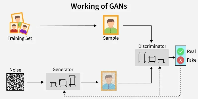
A Generative Adversarial Network (GAN) is a deep learning architecture composed of two competing neural networks, a generator and a discriminator, that learn to create new, realistic data through an adversarial "game". This framework enables the generation of highly convincing synthetic content, such as images, audio, or text, that mimics real-world data.
Components of a GAN
A GAN system comprises two primary deep neural networks that are trained simultaneously:
The Generator: The generator acts like a forger or an artist. It takes a random noise vector as input and transforms it into a synthetic data sample (e.g., an image). Its goal is to produce outputs that are so convincing that the discriminator cannot distinguish them from real data.
The Discriminator: The discriminator acts like a critic or a detective. It is a binary classifier that receives both real data samples (from the training dataset) and fake samples (from the generator). Its job is to evaluate each sample and determine whether it is "real" or "fake," assigning a probability score (e.g., 1 for real, 0 for fake).
The Adversarial Process
The training process is a continuous, zero-sum competition:
Generator attempts forgery: The generator creates a batch of fake data from random noise input.
Discriminator evaluates: The discriminator is presented with both the generator's fake data and actual real data from the training set and classifies each sample as real or fake.
Feedback and improvement:
The discriminator is rewarded for correctly identifying real and fake data, and its parameters are adjusted to improve its classification ability.
The generator is penalized when the discriminator correctly identifies its output as fake. It uses this feedback to adjust its own parameters, learning how to produce more realistic data that is more likely to fool the discriminator in the next round.
This process continues until an equilibrium is reached where the generator becomes so skilled that the discriminator can only guess whether a sample is real or fake with 50% accuracy. At this point, the generator is a highly capable model for creating authentic-looking new data instances.
Key Frameworks in Deep Learning
TensorFlow
TensorFlow is an open-source platform and framework developed by the Google Brain team for building and deploying machine learning (ML) and deep learning models. It is designed for large-scale numerical computation, using a core concept where data "flows" through a graph of mathematical operations in the form of multidimensional arrays called tensors.
Key Features and Ecosystem:
Platform Versatility: TensorFlow models can be trained and run across a wide range of devices, including desktops, server clusters, mobile devices (via TensorFlow Lite), and web browsers (via TensorFlow.js).
Hardware Acceleration: It supports various computing hardware, including CPUs, GPUs, and Google's custom-designed Tensor Processing Units (TPUs) for enhanced performance.
High-Level APIs: TensorFlow integrates seamlessly with Keras, a high-level API that simplifies the process of building and training neural networks.
Comprehensive Tools: The platform includes a rich ecosystem of tools and libraries, such as:
TensorBoard: A visualization suite for inspecting and debugging model graphs and training metrics.
TensorFlow Extended (TFX): A framework for building end-to-end production ML pipelines.
Common Applications:
TensorFlow is used by various companies, including Google itself (for products like Search, Gmail, and Photos), for a wide array of real-world applications:
Image Recognition and Computer Vision: Used in medical image analysis (e.g., detecting diseases from X-rays) and object detection for autonomous systems.
Natural Language Processing (NLP): Powers applications like sentiment analysis in call centers and automatic email response generation.
Speech Recognition: Enables virtual assistants like Google Assistant and Amazon Alexa to understand voice commands.
Recommendation Systems: Utilized by platforms such as Netflix and YouTube to provide personalized content suggestions.
Fraud Detection: PayPal uses TensorFlow for identifying complex and varying fraud patterns.
Keras
Keras is an open-source, high-level Application Programming Interface (API) designed to simplify the process of building, training, and deploying deep learning models. It is known for its user-friendly, modular, and intuitive design, making deep learning more accessible to both beginners and experienced researchers.
Key Concepts
High-Level Abstraction: Keras acts as an abstraction layer (or "wrapper") over lower-level, more complex deep learning frameworks. This allows users to build complex neural networks with minimal, highly readable Python code.
Backend Engines: Originally, Keras was a standalone library that could run on top of several "backend" computation engines, including TensorFlow, Theano, and Microsoft Cognitive Toolkit (CNTK).
Integration with TensorFlow: Keras is now tightly integrated as the official high-level API of TensorFlow (tf.keras). Google recommends that most TensorFlow users utilize the Keras APIs by default.
Multi-Backend Support (Keras 3.0+): With the release of Keras 3.0, the framework has become multi-backend again, offering seamless compatibility with TensorFlow, PyTorch, and JAX, allowing models to move between different computation engines.
Why Use Keras?
Keras is widely adopted for several reasons:
Rapid Prototyping: Its simplicity allows researchers and developers to quickly design and test different network architectures, accelerating the experimentation cycle.
User-Friendliness: Keras prioritizes user experience, offering clear error messages and simple, consistent interfaces that reduce the cognitive load of learning deep learning.
Modularity: Models are built like "Lego blocks" by stacking configurable layers (e.g., dense, convolutional, recurrent layers), which makes it easy to create various model types, from simple feedforward networks to complex computer vision models.
Scalability and Deployment: By leveraging powerful backends like TensorFlow, Keras models can be trained on large clusters of GPUs or TPUs and easily exported to run on various platforms, including web browsers (TensorFlow.js) and mobile devices (TensorFlow Lite).
Keras simplifies the definition of a deep learning model, while the underlying backend (like TensorFlow) handles the complex, low-level mathematical operations and hardware acceleration.
PyTorch
PyTorch is an open-source machine learning framework known for its flexibility, ease-of-use, and dynamic computational graph approach. Originally developed by Meta's AI Research lab and now managed by the Linux Foundation, it has become a leading platform for deep learning research and a growing force in production systems.
Key Features of PyTorch
Pythonic and Intuitive: PyTorch is designed to feel like native Python code, making it easy for developers already familiar with Python and libraries like NumPy to learn and use. This tight integration allows the use of standard Python debugging tools.
Dynamic Computation Graphs: This is a defining feature of PyTorch. Unlike frameworks that require the entire model architecture to be defined statically before running (common in early TensorFlow), PyTorch uses a "define-by-run" approach. The computation graph is built on the fly as code is executed, which provides immense flexibility for experimentation, rapid prototyping, and easier debugging.
Tensors: Tensors are the fundamental data structure in PyTorch, similar to multi-dimensional arrays in NumPy, but with the crucial ability to run on GPUs. This hardware acceleration (via NVIDIA's CUDA platform) significantly speeds up computations for large-scale deep learning tasks.
Automatic Differentiation (Autograd): The built-in autograd engine automatically calculates the gradients needed for backpropagation, which is the core of training neural networks. This eliminates the need for manual gradient computation, streamlining the development process.
Rich Ecosystem: PyTorch offers a robust ecosystem of libraries and tools that support various domains, including computer vision (TorchVision), natural language processing, and speech (TorchAudio).
Real-World Applications:
Leading technology companies and research labs use PyTorch for advanced AI development. Examples include:
Autonomous Driving: Tesla uses PyTorch to train models for its Autopilot system.
Image Generation and Recognition: It powers state-of-the-art image generators (like Stable Diffusion) and image classification systems used in medical analysis and e-commerce.
Natural Language Processing (NLP): Hugging Face's popular transformers library, which is used for building large language models, is built on top of PyTorch.
OpenCV
OpenCV (Open Source Computer Vision Library) is an open-source software library providing a vast collection of tools and algorithms for computer vision, image processing, and machine learning tasks. It is a fundamental tool for enabling machines to "see" and interpret visual data from images and videos, efficiently processing information for a wide range of real-world applications.
Key Features
Integration with NumPy: OpenCV array structures are converted to and from NumPy arrays, an optimized library for numerical operations. This synergy makes it easy to integrate with other scientific computing libraries like SciPy and Matplotlib.
Broad Functionality: It offers over 2,500 algorithms for tasks ranging from basic image manipulation to advanced computer vision projects.
Cross-Platform: It runs on all major operating systems, including Windows, Linux, and macOS.
Deep Learning Integration: It can be integrated with popular deep learning frameworks like TensorFlow and PyTorch for advanced AI tasks.
Common Operations and Applications
OpenCV-Python is used for a variety of tasks in computer vision:
Image and Video Handling: Reading, displaying, and saving images (cv2.imread(), cv2.imshow(), cv2.imwrite()) and videos (cv2.VideoCapture()).
Image Processing: Manipulating images with operations like resizing, rotating, color space conversions (e.g., RGB to grayscale), and blurring/smoothing (e.g., Gaussian, median blur).
Feature Detection: Identifying important features, shapes, and boundaries in an image, such as lines, circles, corners (e.g., Harris Corner Detection), and contours (outlines of objects).
Object Detection and Recognition: Detecting specific objects like faces, eyes, or cars using techniques like Haar cascades or deep learning models.
Augmented Reality and Robotics: Used in applications that require real-time analysis of visual data, such as tracking objects for AR overlays or robot navigation.
Additional Concepts:
Computer Vision
Computer vision is a field of artificial intelligence (AI) that enables computers to interpret and understand the visual world from digital images and videos, effectively replicating human sight and the cognitive abilities associated with it.

- How Computer Vision Works?
Computer vision systems mimic the human visual process through a series of steps, typically involving deep learning models like convolutional neural networks (CNNs).
Image Acquisition: Devices like cameras, drones, or medical scanners capture raw visual data.
Preprocessing: The raw data is refined to enhance quality. This can involve resizing, removing noise, or adjusting contrast.
Feature Extraction: The system identifies key patterns and features, such as edges, shapes, and textures. Lower layers in a neural network might detect basic lines, while deeper layers recognize more complex components like an object's nose or ears.
Analysis and Understanding: Machine learning algorithms process the extracted features to identify and categorize objects or scenes by comparing them against large, pre-trained databases.
Decision and Output: The system provides insights or takes automated action based on its understanding, such as flagging a defect in manufacturing or guiding a self-driving car to stop.
- Key Tasks and Applications:
Computer vision performs various tasks across numerous industries:
Object Detection and Classification: Identifying specific objects within an image and placing them into predefined categories (e.g., distinguishing between a pedestrian, a cyclist, and a car).
Image Segmentation: Dividing an image into distinct regions or labeling every pixel to understand boundaries (e.g., separating the "road" pixels from the "sidewalk" pixels for an autonomous vehicle).
Facial Recognition: A specialized form of object detection that identifies specific individuals by analyzing unique facial features.
Optical Character Recognition (OCR): Extracting text from images or scanned documents and converting it into machine-readable digital text.
Motion Analysis and Tracking: Monitoring the movement of objects over a sequence of video frames, used in surveillance and sports analytics.
Yolo Algorithm
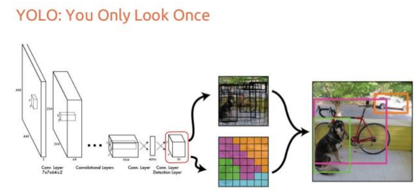
The YOLO (You Only Look Once) algorithm is a highly efficient, single-stage object detection model that revolutionized computer vision by processing entire images in a single pass of a neural network to predict bounding boxes and class probabilities in real time.
The core principle of YOLO is to reframe object detection as a single regression problem, moving directly from image pixels to bounding box coordinates and class probabilities.
The general process involves the following steps:
Grid Division: The input image is divided into an 𝑆×𝑆 grid of cells.
Prediction per Cell: Each grid cell is responsible for detecting objects whose center falls within it. For each cell, it predicts: o Bounding Boxes: Multiple bounding boxes (𝐵boxes) are predicted.
Confidence Score: A confidence score for each box, indicating the likelihood that the box contains an object and the accuracy of the bounding box.
Class Probabilities: A set of conditional class probabilities, indicating which class the object belongs to.
- Non-Maximum Suppression (NMS): This post-processing step filters out redundant or overlapping bounding boxes to yield a final set of high-confidence detections for each object.
Versions of the YOLO Algorithm
YOLOv1 (2015): The original, groundbreaking single-stage model that prioritized speed over the two-stage detectors of its time.
YOLOv2 (2016): Introduced improvements like batch normalization, the use of anchor boxes with k-means clustering, and a new backbone called Darknet-19 to enhance accuracy and the ability to detect more object categories.
YOLOv3 (2018): Used a deeper backbone, Darknet-53, and incorporated a Feature Pyramid Network (FPN) concept for multi-scale detection, significantly improving the performance on small objects.
YOLOv4 (2020): Integrated a vast collection of advanced techniques ("bag of freebies and specials"), such as CSPDarknet53 backbone, the PANet neck, and the Mish activation function, to push the boundaries of efficiency and accuracy.
YOLOv5 (2020): Marked a shift by being the first native PyTorch implementation (maintained by Ultralytics), focusing on a production-ready framework, modularity, and ease of deployment across various devices.
YOLOv6 (2022): Developed by the Meituan team, it introduced an anchor-free approach and a decoupled head design for industry-oriented applications, emphasizing speed and efficiency.
YOLOv7 (2022): Focused on architectural reforms like E-ELAN (extended efficient layer aggregation network) and improved trainable optimizations (auxiliary heads), offering a new state-of-the-art in speed and accuracy.
YOLOv8 (2023): Released by Ultralytics, this version unified support for multiple computer vision tasks (detection, segmentation, pose estimation) and introduced an anchor-free, decoupled-head architecture for greater flexibility and ease of use.
YOLOv9 (2024): A research-focused model that addressed the information bottleneck principle in deep networks, using Programmable Gradient Information (PGI) and the GELAN architecture to achieve high accuracy.
YOLOv10 (2024): Developed by Tsinghua University, this version focused on efficient-accuracy trade-offs by introducing an end-to-end detection head that eliminates the need for Non Maximum Suppression (NMS), reducing latency.
YOLO11 (2024): The latest Ultralytics model, designed for production efficiency with a refined architecture (C3k2 blocks, C2PSA module) to balance speed, accuracy, and task versatility across edge and cloud environments.
YOLOv12 (2024): A community-developed version exploring attention-centric designs (Area Attention module) for further performance enhancements.
YOLO26 (Coming Soon): The next generation model by Ultralytics, focusing on edge optimization and end-to-end NMS-free inference.
How does the Yolo Algorithm work?
The YOLO (You Only Look Once) algorithm works by treating object detection as a single regression problem, processing an entire image through a single convolutional neural network (CNN) to predict bounding boxes and class probabilities simultaneously. This approach allows for real-time performance. The process can be broken down into the following steps:
- Input Image and Grid Division:
The algorithm takes an input image and resizes it to a fixed size (e.g., 448x448 pixels in the original YOLOv1). This image is then divided into an SxS grid (e.g., 7x7) of cells. The core idea is that if the center of an object falls into a specific grid cell, that cell becomes "responsible" for detecting that object.
- Feature Extraction:
The image is passed through a deep Convolutional Neural Network (CNN) backbone (e.g., Darknet in various versions). This network extracts features from the image, which are used by subsequent layers to make predictions.
- Bounding Box and Confidence Prediction:
Each grid cell predicts a fixed number of potential bounding boxes (𝐵 boxes). For each bounding box, it predicts five values:
x, y coordinates: The position of the center of the box relative to the boundaries of the specific grid cell.
w, h (width, height): The width and height of the box relative to the entire image dimensions.
Confidence Score: A score that indicates the likelihood that the box contains an object (objectness score) and the precision of the predicted box's coordinates. If no object is present, the score should be near zero.
- Class Probability Prediction:
Each grid cell also predicts conditional class probabilities for every possible class the model is trained to recognize. These probabilities represent the likelihood of an object belonging to a specific class, given that an object is present in that cell. Note that the original YOLO only predicts one set of class probabilities per cell, regardless of the number of bounding boxes predicted by that cell.
- Final Score Calculation:
During the testing phase, the individual box confidence scores and the conditional class probabilities are multiplied to get class-specific confidence scores for each potential box. This score encodes both the probability of the class and how well the predicted box fits the object.
- Non-Maximum Suppression (NMS):
The network generates numerous overlapping bounding boxes for the same object across different grid cells. To fix this redundancy, a post-processing technique called Non-Maximum Suppression (NMS) is applied. NMS works by:
Selecting the bounding box with the highest class-specific confidence score.
Suppressing all other boxes that significantly overlap with the selected box (determined by a threshold using the Intersection over Union, or IoU, metric).
The final output is a refined list of high-confidence bounding boxes, each correctly localizing and classifying a single object within the image.
Thank you for reading the article! 😊


